WORK IN PROGRESS
This tutorial will explain how to calculate facial sexual dimorphism (SD) in a set of 2D faces, using a vector method (e.g.,[1–3]) and linear discriminant analysis (e.g.,[4]).
Read and prep landmark data
path_to_tem <- system.file("extdata", "tem", package="facefuns")

shapedata <- facefuns(data = read_lmdata(lmdata = path_to_tem,
                                         plot = FALSE),
                      remove_points = "frlgmm",
                      pc_criterion = "broken_stick",
                      plot_sample = FALSE,
                      quiet = TRUE)
In addition, we’ll also need to know which of the faces in our sample are female, and which are male.
1. Vector scores: calc_(shape)vs
facefuns::calc_vs calculates sexual dimorphism by computing an n-dimensional vector between the average female and the average male shape, and then projecting each face onto this vector. Scores are scaled so that a score of 0 corresponds to the average female, and a score of 1 to the average male shape; a negative score, e.g., would thus indicate a hyperfeminine face.
You can use calc_vs to calculate vector scores from a data frame or matrix of principal component scores (see help(calc_vs)), or calc_shapevs to calculate them from the Procrustes-aligned templates in the facefuns output.
calc_shapevs takes three arguments, all of which should be a data frame or matrix with specimen as rows, and PC scores as columns:
-
facefuns_obj: Output fromfacefuns::facefuns -
anchor1_index: Vector specifying indices of faces that will constitute lower anchor point
-
anchor2_index: Vector specifying indices of faces that will constitute upper anchor point
We get the index of which faces in our array of Procrustes-aligned faces are female/male by testing which IDs have a corresponding entry in the info table for which sex == female/male
fem_i <- gsub("^ID=","", dimnames(shapedata$aligned)[[3]]) %in%
  LondonSet_info$face_id[which(LondonSet_info$face_sex == "female")]

mal_i <- gsub("^ID=", "", dimnames(shapedata$aligned)[[3]]) %in%
  LondonSet_info$face_id[which(LondonSet_info$face_sex == "male")]
Now, we can run our function:
sd_vector <- calc_shapevs(shapedata, fem_i, mal_i)calc_(shape)vs will return a tibble that has two columns, id and VS:
head(sd_vector)
#> # A tibble: 6 x 2
#>   id          VS
#>   <chr>    <dbl>
#> 1 001   -1.06
#> 2 002    0.00299
#> 3 003   -0.250
#> 4 004    0.855
#> 5 005    0.548
#> 6 006    0.582
LondonSet_info %>%
  dplyr::left_join(sd_vector, by = c("face_id" = "id")) %>%
  ggplot(aes(x = VS, color=face_sex, fill = face_sex)) +
  geom_histogram(binwidth = .1) +
  theme_bw()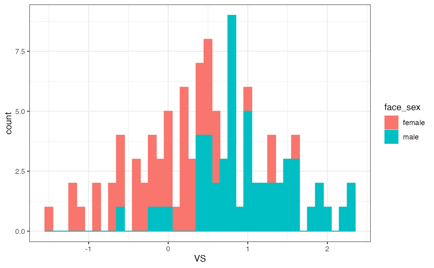
Note: calculating vector scores within- and out-of-set
If your current sample is small, but you have a larger sample at hand that was delineated with the same landmarks or a compatible sub-/superset, you could use that bigger sample to build your shape PCA model and construct the sexual dimorphism vector, and then project faces from the smaller sample onto that vector. You can find an example here (to be updated and added to this vignette in the future).
Note: calculating sexual dimorphism from symmetrized faces
Two-dimensional images are strongly affected by head posture, which is reflected in the fact that in 2D sets, the first principal components usually show shape associated with heads being tilted up/down, or heads being turned left/right. While it is not possible to “correct” for up/down head postures (plus shape differences associated with an upward-/downward-tilt overlap with those of sexual dimorphism), slight asymmetries due to a left/right tilt could be “remedied” by symmetrizing faces.
You could either symmetrize templates before submitting them to facefuns (using facefuns::symm_templates) which has the added benefit that it’s very little fuss to plot the PCs on which the scores are based; or you could do so by using the option symm = TRUE in calc_shapevs.
Symmetrizing works by mirroring each landmark template, and calculating the mean between the original and mirrored template. After mirroring, the landmarks need to be relabeled - what used to be point 0 (right pupil) in the original template, is point 1 (the left pupil) after mirroring.
Unfortunately, this information needs to be manually entered, and will very much depend on the landmark template you want to mirror. For the set of 132 landmarks used throughout the examples in facefuns, this info is stored in mirroredlandmarks.
If symm = TRUE, calc_shapevs will first symmetrize the faces, re-conduct a GPA and PCA on these symmetrized templates, and then run calc_vs.
data("mirroredlandmarks")

sd_vector_symm <- calc_shapevs(shapedata, fem_i, mal_i, symm = TRUE, mirroredlandmarks = mirroredlandmarks)
head(sd_vector_symm)
#> # A tibble: 6 x 2
#>   id        VS
#>   <chr>  <dbl>
#> 1 001   -0.990
#> 2 002    0.121
#> 3 003   -0.205
#> 4 004    0.748
#> 5 005    0.555
#> 6 006    0.526

LondonSet_info %>%
  dplyr::left_join(sd_vector_symm, by = c("face_id" = "id")) %>%
  ggplot(aes(x = VS, color=face_sex, fill = face_sex)) +
  geom_histogram(binwidth = .1) +
  theme_bw()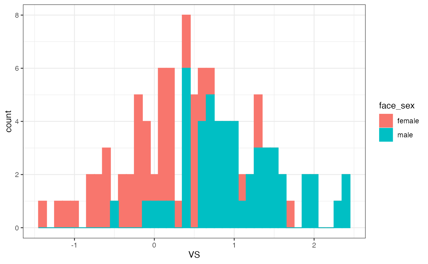
2. Discriminant scores: calc_ds
Another way to calculate sexual dimorphism is by employing a linear discriminant analyses to predict group membership.
calc_ds first conducts a (forward) stepwise variable selection and then carries out a linear discriminant analysis. It takes two arguments:
-
data: A data frame or matrix with specimen as rows, and PCs as columns. Can also contain an additional column that defines group membership. -
group_info: Either a data frame with two columns (col 1 = id matching the rownames in data; col 2 = group), or a single numeric value indexing the column in data that contains group membership info
For this example, we’ll specify group membership with a separate data frame.
group_info <- LondonSet_info %>%
  dplyr::select(face_id, face_sex)

sd_discrim <- calc_ds(shapedata$pc_scores, group_info = group_info)
Like calc_vs, calc_ds will return a tibble that has two columns, in this case id and DS:
head(sd_discrim)Compare vector and discriminant scores
compareSD <- LondonSet_info %>%
  dplyr::left_join(sd_vector, by = c("face_id" = "id")) %>%
  dplyr::left_join(sd_discrim, by = c("face_id" = "id"))

compareSD %>%
  dplyr::group_by(face_sex) %>%
  dplyr::summarise(mean_vs = round(mean(VS), 3),
                   mean_ds = round(mean(DS), 3))
#> # A tibble: 2 x 3
#>   face_sex mean_vs mean_ds
#>   <chr>      <dbl>   <dbl>
#> 1 female         0   -1.45
#> 2 male           1    1.34

compareSD %>%
  ggplot(aes(x = VS, y = DS)) +
  geom_point(aes(color = face_sex)) +
  geom_smooth(method='lm', formula = y ~ x, color = "purple") +
  theme_bw()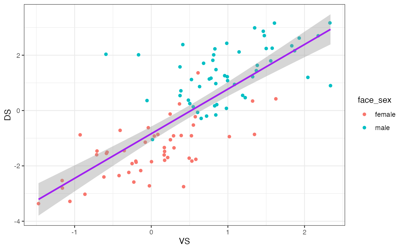

References
1. Holzleitner, I. J., Hunter, D. W., Tiddeman, B. P., Seck, A., Re, D. E., & Perrett, D. I. (2014). Men’s facial masculinity: When (body) size matters. Perception, 43, 1191–1202. https://doi.org/10.1068/P7673
2. Komori, M., Kawamura, S., & Ishihara, S. (2011). Multiple mechanisms in the perception of face gender: Effect of sex-irrelevant features. Journal of Experimental Psychology-Human Perception and Performance, 37, 626–633. https://doi.org/10.1037/A0020369
3. Valenzano, D. R., Mennucci, A., Tartarelli, G., & Cellerino, A. (2006). Shape analysis of female facial attractiveness. Vision Research, 46, 1282–1291. https://doi.org/10.1016/j.visres.2005.10.024
4. Scott, I. M. L., Pound, N., Stephen, I. D., Clark, A. P., & Penton-Voak, I. S. (2010). Does masculinity matter? The contribution of masculine face shape to male attractiveness in humans. PLoS ONE, 5. https://doi.org/10.1371/journal.pone.0013585